Propane parameter estimation#
Evidence: calibration. Fit three PC-SAFT pure-fluid parameters to six
observations, saturation pressure and saturated liquid mass density at
210, 270 and 330 K. Start from gross-2001-propane/3, Gross and Sadowski (2001),
Table 2 (paper).
The observations are Glos, Kleinrahm and Wagner (2004), Table 2
(paper), retained as
engine/tests/cases/pure-saturation-regression/inputs/source/propane-baseline.csv.
Zotero NF5HJCV7 is metadata only; no local PDF attachment is claimed.
The official NIST/TRC ThermoML record
provides the machine-readable measurements. The retained source record
engine/tests/cases/2004-glos/inputs/source/glos-2004-propane-saturation.yaml
documents the compact factual extraction and source-specific use basis.
Source pressures in kPa were multiplied by exactly 1000 to obtain the Pa
values read from the teaching CSV; mass densities remain in kg/m³.
Read the inputs#
Use a repository checkout with the environment described in the installation guide. The wheel alone does not contain these data. All density, association, equilibrium and parameter-fit iterations below run in the native Engine.
from pathlib import Path
import csv
import pandas as pd
from IPython.display import display
from epcsaft import (
    Parameters,
    Pure,
)
from epcsaft import equilibrium as eq, regression as rg

pd.set_option("display.max_columns", None)
pd.set_option("display.max_colwidth", None)

ROOT = next(
    folder
    for folder in (Path.cwd(), *Path.cwd().parents)
    if (folder / "ARCHITECTURE.yaml").is_file()
)
PACKETS = ROOT / "data" / "packets"
Declare observations, coordinates and one native fit#
Each observation uses a zero-vapor-amount saturation declaration. Log-ratio residuals have unit weight, a calibration choice rather than source measurement uncertainty. Coordinates use origin/scale/bounds:
Parameter |
Origin |
Scale |
Bounds |
|---|---|---|---|
Dispersion energy/k / K |
221 |
10 |
150–260 |
Segment count / 1 |
1.9489 |
0.1 |
1.5–2.5 |
Segment diameter / Å |
3.7209 |
0.1 |
3–4.2 |
The native budget is 100 iterations and 60 s, with one published-packet start. Require usable parameters, lower cost, and independent native re-evaluation of all fitted predictions within 10⁻¹⁰ relative.
start = Parameters.from_json(
    PACKETS / "gross-2001-propane/3/parameters/parameters.json", components=["propane"]
)
rows = list(
    csv.DictReader(
        (
            ROOT
            / "engine/tests/cases/pure-saturation-regression/inputs/source/propane-baseline.csv"
        ).open()
    )
)
observations = []
for row in rows:
    problem = eq.Problem(
        T=float(row["temperature_k"]),
        P=eq.Free(float(row["saturation_pressure"])),
        feed=eq.Amounts({"propane": 1}),
        phases=[
            eq.Phase("L", kind="liquid"),
            eq.Phase("V", kind="vapor", amount=eq.Pinned(0)),
        ],
        row_tolerance=1e-10,
    )
    observations += [
        rg.saturation_pressure_observation(
            start,
            component="propane",
            T=float(row["temperature_k"]),
            observed=float(row["saturation_pressure"]),
            form="log_ratio",
        ),
        rg.observation(
            start,
            "phase_density",
            problem,
            observed=float(row["saturated_liquid_mass_density"]),
            phase="L",
            form="log_ratio",
            mass_basis=True,
        ),
    ]
coordinates = [
    rg.coordinate(
        start, [(name, "propane", 1)], origin=origin, scale=scale, bounds=bounds
    )
    for name, origin, scale, bounds in [
        ("dispersion_energy_over_k", 221, 10, (150, 260)),
        ("segment_count", 1.9489, 0.1, (1.5, 2.5)),
        ("segment_diameter", 3.7209, 0.1, (3, 4.2)),
    ]
]
fit_result = rg.fit(
    start,
    coordinates,
    observations,
    controls=rg.FitControls(maximum_iterations=100, maximum_elapsed_time_seconds=60),
)
assert fit_result.usable, fit_result.message
assert fit_result.final_cost < fit_result.initial_cost
fitted_parameters = rg.fitted_parameters(start, fit_result)
predictions = [
    rg.predict(Pure(fitted_parameters), observation).value
    for observation in observations
]
assert all(
    (
        abs(a - b) < 1e-10 * max(abs(a), 1)
        for a, b in zip(predictions, fit_result.predictions)
    )
)
values = dict(
    physical=fit_result.physical,
    initial_cost=fit_result.initial_cost,
    final_cost=fit_result.final_cost,
    iterations=fit_result.iterations,
    predictions=fit_result.predictions,
    residuals=fit_result.residuals,
    covariance_rank=fit_result.covariance.rank,
    covariance_assumption=fit_result.covariance.assumption,
    observed=[o.observed for o in observations],
)
values["prediction_round_trip_relative_error"] = max(
    (abs(a - b) / abs(a) for a, b in zip(predictions, fit_result.predictions))
)
assert values["prediction_round_trip_relative_error"] <= 1e-10
display(
    pd.DataFrame(
        {
            "Observation": ["Pressure / Pa", "Liquid density / kg m^-3"] * 3,
            "Temperature / K": [210, 210, 270, 270, 330, 330],
            "Observed": values["observed"],
            "Fitted prediction": values["predictions"],
            "Log-ratio residual / 1": values["residuals"],
        }
    )
)
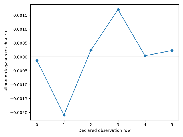
| Observation | Temperature / K | Observed | Fitted prediction | Log-ratio residual / 1 | |
|---|---|---|---|---|---|
| 0 | Pressure / Pa | 210 | 36032.000 | 3.602740e+04 | -0.000128 |
| 1 | Liquid density / kg m^-3 | 210 | 604.594 | 6.033307e+02 | -0.002092 |
| 2 | Pressure / Pa | 270 | 430425.000 | 4.305303e+05 | 0.000245 |
| 3 | Liquid density / kg m^-3 | 270 | 532.853 | 5.337605e+02 | 0.001702 |
| 4 | Pressure / Pa | 330 | 1983000.000 | 1.983084e+06 | 0.000042 |
| 5 | Liquid density / kg m^-3 | 330 | 434.869 | 4.349694e+02 | 0.000231 |
Inspect calibration residuals#
Rows alternate saturation pressure and liquid density at the three temperatures. These are residuals against the same measurements used in the fit.
from io import BytesIO
from IPython.display import Image
import matplotlib.pyplot as plt

plt.plot(range(6), values["residuals"], marker="o")
plt.axhline(0, color="black")
plt.xlabel("Declared observation row")
plt.ylabel("Calibration log-ratio residual / 1")
buffer = BytesIO()
plt.tight_layout()
plt.savefig(buffer, format="png")
plt.close()
display(Image(data=buffer.getvalue()))
display(pd.DataFrame({
    "Dispersion energy/k / K": [values["physical"][0]],
    "Segment count / 1": [values["physical"][1]],
    "Segment diameter / Å": [values["physical"][2]],
}))
display(pd.DataFrame([{
    "Initial cost / 1": values["initial_cost"],
    "Final cost / 1": values["final_cost"],
    "Iterations / 1": values["iterations"],
    "Covariance rank / 1": values["covariance_rank"],
    "Covariance assumption": values["covariance_assumption"],
    "Prediction round-trip relative error / 1": values["prediction_round_trip_relative_error"],
}]))
| Dispersion energy/k / K | Segment count / 1 | Segment diameter / Å | |
|---|---|---|---|
| 0 | 208.511249 | 1.996456 | 3.619429 |
| Initial cost / 1 | Final cost / 1 | Iterations / 1 | Covariance rank / 1 | Covariance assumption | Prediction round-trip relative error / 1 | |
|---|---|---|---|---|---|---|
| 0 | 0.000014 | 0.000004 | 5 | 3 | unit-variance weighted residuals, independent errors and a regular local linearization at an interior point; multiply by variance_factor for an unknown common variance; no claim under bounds, rank deficiency or model discrepancy | 3.379998e-15 |
Meaning and limits#
This is calibration against direct measurements. It supplies no independent validation set or new predictive accuracy floor. The printed covariance rank and assumption describe a local linearized calculation conditional on the declared weights and residual model. They do not establish global identifiability or predictive uncertainty. The fitted values are a tutorial result, not a newly adopted canonical parameter set.