Halite solubility#
Evidence: physical comparison, with numerical balance and complementarity checks. At 298.15 K and 101,325 Pa, add 5, 6.5 and 7.5 mol NaCl to 1 kg water.
The liquid uses Held et al. (2014), Tables 1–3
(paper), specifically
held-2014-strategy2/1. Clarke and Glew (1985)
(paper), Table 34, supplies dissolution
ΔG = −9038.7 J/mol; Table 17A supplies the measured 6.1476 mol/kg solubility.
The retained PHREEQC pitzer.dat record supplies 27.1 × 10⁻⁶ m³/mol solid
molar volume, as documented in the existing halite reference case.
Read the inputs#
Use a repository checkout with the environment described in the installation guide. The wheel alone does not contain these data. All density, association, equilibrium and parameter-fit iterations below run in the native Engine.
from pathlib import Path
import pandas as pd
from IPython.display import display
from epcsaft import (
    Parameters,
    Mixture,
)
from epcsaft import equilibrium as eq

pd.set_option("display.max_columns", None)
pd.set_option("display.max_colwidth", None)

ROOT = next(
    folder
    for folder in (Path.cwd(), *Path.cwd().parents)
    if (folder / "ARCHITECTURE.yaml").is_file()
)
PACKETS = ROOT / "data" / "packets"


def equilibrium_values(solved):
    """Keep the returned physical state and the equation residuals together."""
    assert solved.success, solved.message
    assert solved.requested_tolerance_met
    assert solved.classified_residuals
    residual = max(map(abs, solved.classified_residuals), default=0)
    assert residual <= 1e-10
    return dict(
        temperature_K=solved.temperature,
        pressure_Pa=solved.pressure,
        amounts_mol=solved.amounts,
        mole_fractions=solved.mole_fractions,
        molar_densities_mol_m3=solved.molar_densities,
        residual=residual,
        linear_solver=solved.linear_solver,
    )
Declare a stoichiometric solid#
NaCl(s) contains one sodium ion and one chloride ion. The source standard is infinite dilution on a 1 mol/kg molality basis at 101,325 Pa. Declare the accepted scalar ln K = 3.6461705031852696 only at 298.15 K; no temperature law is inferred. The Engine owns reference conversion and solid complementarity.
For each feed, require sodium plus solid balance within 10⁻¹⁰ times feed and classified residuals at most 10⁻¹⁰. An absent solid has negative saturation index; each present solid must have index within 10⁻¹⁰ of zero. Saturated liquid molalities must agree within 10⁻⁸ mol/kg. Retain the existing 3% relative comparison with the measured solubility.
model = Mixture(
    Parameters.from_json(
        PACKETS / "held-2014-strategy2/1/parameters/parameters.json",
        components=["water", "sodium-cation", "chloride-anion"],
    )
)
ln_k = 3.6461705031852696
law = eq.ReactionLogPolynomial(
    ln_k, 0, 0, 0, 298.15, 298.15, 298.15, "molality-infinite-dilution"
)
solid = eq.Solid(
    "halite",
    formula={"sodium-cation": 1, "chloride-anion": 1},
    correlation=law,
    reference=eq.ReactionReference(
        eq.ReferenceSourceBasis.CommonMolalityInfiniteDilution, 101325
    ),
    molar_volume_m3_per_mol=2.71e-05,
)
solved = []
for feed in (5.0, 6.5, 7.5):
    problem = eq.Problem(
        T=298.15,
        P=101325,
        phases=[eq.Phase("L", kind="liquid")],
        solids=[solid],
        feed=eq.Molalities(
            {"sodium-cation": feed, "chloride-anion": feed},
            solvent=["water"],
            solvent_mass_kg=1,
        ),
        neutral_reference=eq.NeutralReference(
            solvent="water",
            solute_molality_ratios={"sodium-cation": 1, "chloride-anion": 1},
            standard_molality_mol_per_kg=1,
        ),
    )
    equilibrium_result = eq.solve_equilibrium(model, problem)
    solved_values = equilibrium_values(equilibrium_result)
    molality = equilibrium_result.amounts[0] * equilibrium_result.mole_fractions[1]
    assert abs(molality + equilibrium_result.solid_amounts[0] - feed) <= 1e-10 * feed
    solved_values.update(
        feed_mol_kg=feed,
        liquid_molality_mol_kg=molality,
        solid_amount_mol=equilibrium_result.solid_amounts[0],
        saturation_index=equilibrium_result.solid_affinity_decades[0],
    )
    solved.append(solved_values)
assert abs(solved[1]["liquid_molality_mol_kg"] / 6.1476 - 1) < 0.03
assert (
    abs(solved[1]["liquid_molality_mol_kg"] - solved[2]["liquid_molality_mol_kg"])
    < 1e-08
)
assert solved[0]["solid_amount_mol"] == 0 and solved[0]["saturation_index"] < 0
assert all((abs(row["saturation_index"]) < 1e-10 for row in solved[1:]))
values = dict(
    ln_K=ln_k,
    solves=solved,
    source_solubility_mol_kg=6.1476,
    relative_discrepancy=solved[1]["liquid_molality_mol_kg"] / 6.1476 - 1,
)
display(
    pd.DataFrame(solved)[
        [
            "feed_mol_kg",
            "liquid_molality_mol_kg",
            "solid_amount_mol",
            "saturation_index",
            "residual",
        ]
    ]
)
| feed_mol_kg | liquid_molality_mol_kg | solid_amount_mol | saturation_index | residual | |
|---|---|---|---|---|---|
| 0 | 5.0 | 5.000000 | 0.000000 | -0.302933 | 3.089760e-14 |
| 1 | 6.5 | 6.298905 | 0.201095 | 0.000000 | 1.157608e-14 |
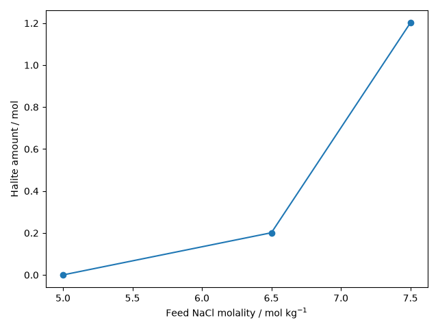
| 2 | 7.5 | 6.298905 | 1.201095 | 0.000000 | 8.133975e-15 |
Show excess salt entering the solid#
Each point is a computed feed case. The connecting line guides the eye.
from io import BytesIO
from IPython.display import Image
import matplotlib.pyplot as plt

plt.plot(
    [solved["feed_mol_kg"] for solved in values["solves"]],
    [solved["solid_amount_mol"] for solved in values["solves"]],
    marker="o",
)
plt.xlabel("Feed NaCl molality / mol kg$^{-1}$")
plt.ylabel("Halite amount / mol")
buffer = BytesIO()
plt.tight_layout()
plt.savefig(buffer, format="png")
plt.close()
display(Image(data=buffer.getvalue()))
display(pd.DataFrame(values["solves"])[[
    "temperature_K", "pressure_Pa", "amounts_mol", "mole_fractions",
    "molar_densities_mol_m3", "linear_solver",
]].rename(columns={
            "temperature_K": "Temperature / K",
            "pressure_Pa": "Pressure / Pa",
            "amounts_mol": "Phase amounts / mol",
            "mole_fractions": "Mole fractions / 1",
            "molar_densities_mol_m3": "Phase densities / mol m^-3",
            "residual": "Maximum classified residual / 1",
            "linear_solver": "Linear solver",
        }))
display(pd.DataFrame([{
    "ln K / 1": values["ln_K"],
    "Source solubility / mol kg^-1": values["source_solubility_mol_kg"],
    "Relative discrepancy / 1": values["relative_discrepancy"],
}]))
| Temperature / K | Pressure / Pa | Phase amounts / mol | Mole fractions / 1 | Phase densities / mol m^-3 | Linear solver | |
|---|---|---|---|---|---|---|
| 0 | 298.15 | 101325.0 | [65.50843506179197] | [0.8473479027461528, 0.07632604862692356, 0.07632604862692356] | [58395.801921021724] | mumps |
| 1 | 298.15 | 101325.0 | [68.1062442800043] | [0.8150271043221954, 0.09248644783890235, 0.09248644783890235] | [59045.75616417084] | mumps |
| 2 | 298.15 | 101325.0 | [68.10624428000433] | [0.815027104322195, 0.09248644783890253, 0.09248644783890253] | [59045.75616417084] | mumps |
| ln K / 1 | Source solubility / mol kg^-1 | Relative discrepancy / 1 | |
|---|---|---|---|
| 0 | 3.646171 | 6.1476 | 0.024612 |
Meaning and limits#
The comparison covers one salt, one temperature and one source convention. These concentrations exceed the packet’s broader assessment ending at 4.5 mol/kg; the existing solubility reference case supplies this bounded use. The 3% criterion is a comparison criterion, not a measurement uncertainty or general salt-accuracy claim. Keep the packet’s private scientific verification use basis; this example does not relicense its source collection.